This report describes a data pipeline and a price-direction model for the EA Sports FC Ultimate Team card market. It covers the data, the way the prediction problem is framed, the validation method used to avoid over-stating the result, and the measured performance, reported both as a statistical score and as a simulated trading return. The model is trained on two seasons of the game and tested on a third that it never sees during training. It beats the relevant baselines, the result holds on the unseen season, and a portfolio simulation produces a positive return after market fees. A short run of real trades placed on the model's calls is reported alongside the simulation. The final section sets out where the model has no skill.
Background
Ultimate Team is the card-collecting mode in EA Sports FC. Each real footballer has one or more cards, every card has a coin price set by a player-to-player market, and those prices move daily with promotions, squad-building challenges, and ordinary supply and demand. Cards are traded for profit.
The prediction task is deliberately narrow: given a card and where it is in its lifecycle, will its price be meaningfully higher, lower, or about the same roughly two weeks later? A prediction that is better than chance can be traded on.
Data
The raw data comes from public FUT data sources. Card information and current-season price history come from FUT.GG and price history for the two older seasons comes from FUTBIN.
Across three game years (FC24, FC25, FC26) the dataset covers roughly 72,000 distinct cards and about 17.8 million daily price points, together with each card's attributes (rating, position, stat line, playstyles, and so on). The model uses price history, the daily time series of each card's value.
Data platform
The data is held in a Databricks lakehouse, which handles everything after the raw data lands: cleaning, joining, building model inputs, training, and the dashboards. The design follows the standard medallion layout:
- Raw payloads are stored exactly as received, so any later stage can be rebuilt from source.
- Each source is cleaned and standardized on its own (fields typed, duplicates removed, the price series expanded to one row per day).
- Sources are combined only at the final layer, into a single card-centric view and a set of model tables.
Every result below is tied to a specific version of the underlying data, and each model run records the data versions it used, so any figure can be traced back to the rows that produced it. The charts in this report are read directly from these tables by Databricks dashboards, so the visuals and the numbers share one source.
Problem formulation
The model does not predict the future coin price directly. It predicts the size of the move: the change in price over 14 days, expressed as a log-return (the natural log of the future price divided by the current price, which makes increases and decreases symmetric and additive). At decision time this number is converted into an action: if the predicted move is large enough to clear the market's 5% sales tax, the card is a buy; otherwise it is a hold or avoid.
Predicting the move rather than the price is deliberate. Card prices span several orders of magnitude, from a few hundred coins to over a million, so a model trained on absolute prices spends its effort fitting the handful of most expensive cards (where the raw error is largest) and is graded on a scale that has nothing to do with whether a trade is worth making. Expressing the target as a per-card relative move puts every card on the same footing, regardless of how much it costs, while preserving the magnitude needed for the later profit simulation.
Further choices:
- The model is cold-start: it is designed to work on cards that are still new and have little price history, since that is when a trading decision is most valuable.
- Decisions are made weekly, on a fixed day, so predictions are spaced out rather than overlapping daily.
- A single model is used for all cards, with card age included as a feature, rather than one model per card or per year.
- The model is trained on FC24 and FC25 and tested on FC26, a season it never sees during training.
Evaluation method
This section sets out the steps taken to keep the reported performance honest, since time-series prediction of this kind is prone to over-optimistic results.
Choice of metric. Most cards mostly hold. If "hold" is the correct answer 60% of the time, a model that always predicts "hold" is 60% accurate while carrying no information, so accuracy is not a useful score here. The headline metric is the Matthews correlation coefficient (MCC), which credits correct up, hold, and down calls relative to how often each outcome actually occurs. It ranges from 0 (no better than chance) toward 1. The values are small next to a raw accuracy figure, which is expected for a problem with this kind of skewed class balance.
Baselines. Before any model was trained, a set of baselines (the "floors") was established, and beating them was set as the minimum requirement:
- Always predict the most common outcome.
- Assume the price continues its recent move (momentum).
- The lifecycle prior: for cards of a given type and age, predict the average move that category of card typically makes.
The lifecycle prior is the meaningful bar. It scores an MCC of about 0.049 and returns about +0.014 coins per trade after tax by trading selectively. A model that cannot beat predicting the typical move for similar cards adds no value.
Avoiding information leakage (purge and embargo). The data is split into a training part and a test part in time order: earlier weeks are used for training, later weeks for testing, and the window rolls forward (walk-forward validation). The complication is that each label looks 14 days ahead, so a training example near the end of the training window and a test example near the start of the test window can overlap in real time, which lets information from the test period enter training. To prevent this, a buffer of examples is removed on both sides of each split, wide enough to cover the 14-day look-ahead (a 31-day gap), and all cards belonging to one player are kept on the same side of the split. This reduces the amount of usable data but is necessary for the score to be valid.
In addition, every feature is computed only from information available on or before the decision day, and this constraint is asserted during the build so that no feature can read future data.
Results
The model was developed in stages, simplest first, with each stage required to beat the one below it. Each stage must clear two bars: the statistical one (MCC) and the economic one (coins per trade, after tax). "CV" denotes the walk-forward cross-validation on the training seasons; "FC26" denotes the held-out test season.
| Strategy | CV MCC | CV coins/trade | FC26 MCC | FC26 coins/trade |
|---|---|---|---|---|
| Lifecycle prior (the bar) | 0.049 | +0.014 | 0.088 | +0.047 |
| Ridge regression | 0.071 | +0.052 | 0.136 | +0.075 |
| Gradient-boosted trees (A) | 0.113 | +0.109 | 0.204 | +0.118 |
| Gradient-boosted trees (B) | 0.123 | +0.120 | 0.202 | +0.117 |
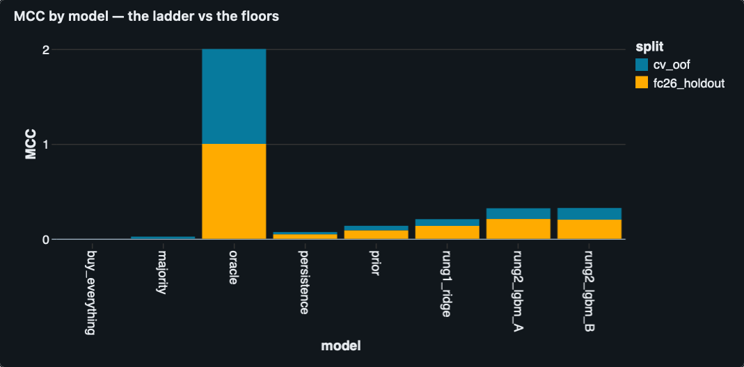
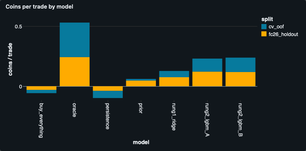
Several points follow from the table. The linear model (ridge regression) already clears the bar, which shows that a per-card prediction beats the category-average prediction. The gradient-boosted trees roughly double the result again. The trees were run in two configurations to locate the source of the gain: configuration A changes only the model form (trees capture curves and interactions that a linear model cannot) using the same inputs, while configuration B adds higher-cardinality features (league and nation). Almost all of the improvement comes from the model form rather than the added features; the additional features contribute a little, and that contribution does not carry to the new season, so it is treated as secondary.
The most important result is that every model scored higher on FC26, the unseen season, than in cross-validation. This is the opposite of what over-fitting would produce, and indicates that the lifecycle pattern recurs from one season to the next.
Trading simulation
MCC measures the quality of the calls but not their effect on a balance. A portfolio simulation runs the model forward as a trader would, entirely on FC26 (the out-of-sample season).
The rules match the constraints a real trader faces. Beginning from a coin balance, each week the highest-ranked cards are bought, held for 14 days, sold, and charged the 5% sales tax, with proceeds reinvested. Because a single card cannot be bought in unlimited quantity, a cap limits how much is placed in any one card. Three comparisons were run through the same process: a random buyer, a buy-everything buyer, and the lifecycle-prior strategy.
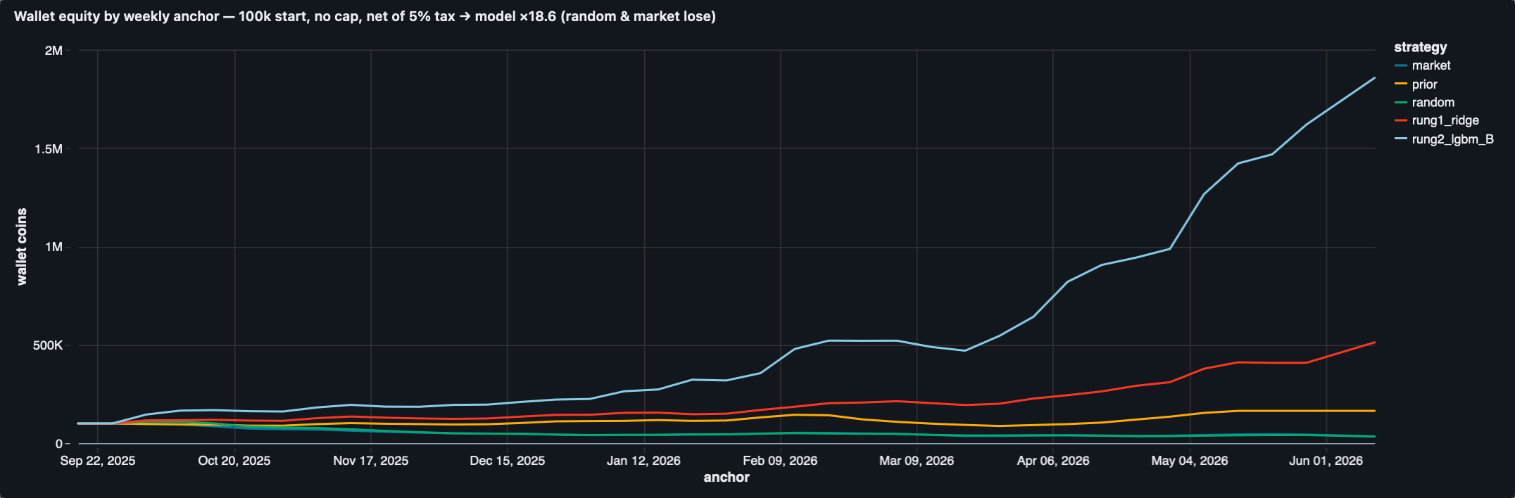
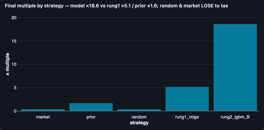
Starting from 100,000 coins, the model grows the balance about 18-fold over the season with no liquidity limit, and by roughly 7× down to about 2× once realistic per-card caps apply (a tighter cap gives a lower multiple, as expected). The random and buy-everything strategies both lose coins. This last point is significant: the sales tax penalizes indiscriminate trading, so being active in the market is not itself the source of return. Selection is.
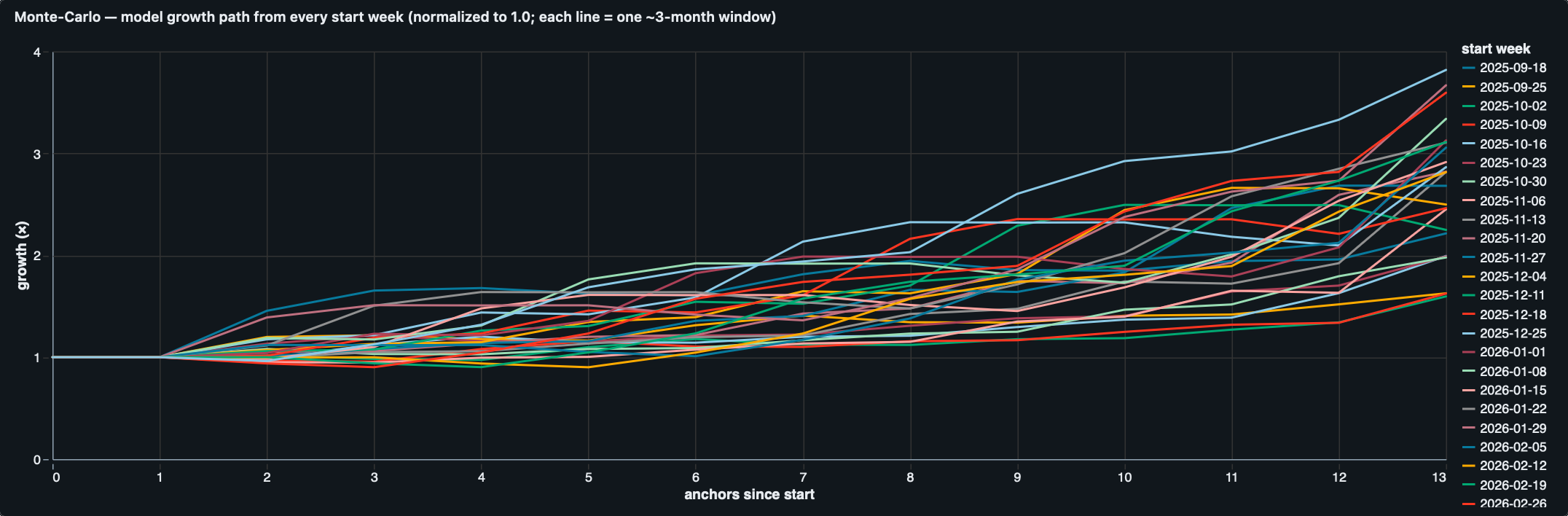
A reasonable concern is that FC26 may simply have been a favorable season. To test this, the simulation was run over many overlapping three-month windows across the year, and within each window the random buyer was run hundreds of times with different seeds to map the distribution of outcomes under random selection. The model's worst three-month window exceeded the best of those random runs, and in every window it landed above the 95th percentile of the random distribution. A result whose worst case beats the best case of random selection is not attributable to chance.
Trading the model live
A simulation is not a market. To check that the model's calls survive contact with the real thing, I traded them myself with real coins on the live FC26 market over three weeks in July 2026.
The method was to take the model's weekly buy list, buy those cards on the open market at whatever price they were actually available for, and close each position inside the model's 14-day horizon. Exits were my own judgement within that window rather than a mechanical sale on day 14. Every figure below is net of the 5% sales tax and comes from the actual transaction record.
| Week | Trades | Deployed | Proceeds | Net profit | Return |
|---|---|---|---|---|---|
| 6 Jul | 7 | 149,250 | 286,250 | +122,687.5 | +82.2% |
| 13 Jul | 12 | 173,350 | 291,000 | +103,100 | +59.5% |
| 16–20 Jul | 7 | 189,200 | 294,000 | +90,100 | +47.6% |
| Total | 26 | 511,800 | 871,250 | +315,887.5 | +61.7% |
Across the 26 completed trades the mean return was +75% per trade, the average holding period was 3.9 days, and the individual outcomes ranged from +1.8% to +256%.
One observation is worth separating from the numbers. The model's picks did not reliably peak on day 14; they tended to rise at some point inside the 14-day window and were often well off that high by the time the window closed. The backtest marks every position at day 14 by construction, so it measures the wrong point on the path — it charges the model for a drawdown that a trader watching the position would not have taken. This suggests the day-14 figures understate what the same signal is worth under a discretionary exit. It is a hypothesis produced by trading the model, not a result: testing it properly means re-running the backtest against the best exit available in the window, and that has not been done.
How much weight this deserves. Not much on its own, and it should not be read as a second validation of the model. It is 26 trades by one person over three weeks, self-reported, with no control arm running alongside it, in a stretch of the calendar unusually thick with promotions. The exits were discretionary, so the result reflects my timing as well as the model's selection and the two cannot be separated from this record. The per-trade return is far above the +0.118 the backtest reports for FC26, and that gap is explained by the different exit rule, the small sample and the favourable window rather than by the model being better than measured. The out-of-sample season and the randomisation test remain the evidence; this section is a field check that the calls are tradable at real prices, which a backtest cannot demonstrate.
View the full trade log — 26 trades
| Card | Rating | Promo | Bought | Buy | Sold | Sell | Profit after tax |
|---|---|---|---|---|---|---|---|
| Sergiño Dest | 86 | Joga Bonito | 6 Jul | 23,000 | 14 Jul | 32,750 | +8,112.5 |
| Sergiño Dest | 86 | Joga Bonito | 6 Jul | 23,000 | 17 Jul | 50,000 | +24,500 |
| Sergiño Dest | 86 | Joga Bonito | 6 Jul | 28,000 | 17 Jul | 50,000 | +19,500 |
| Sergiño Dest | 86 | Joga Bonito | 6 Jul | 28,000 | 14 Jul | 30,000 | +500 |
| Barbra Banda | 86 | Winter Wildcards | 6 Jul | 16,250 | 9 Jul | 41,000 | +22,700 |
| Doucouré | 87 | Time Warp | 6 Jul | 14,000 | 6 Jul | 52,500 | +35,875 |
| Mario Götze | 88 | Time Warp | 6 Jul | 17,000 | 10 Jul | 30,000 | +11,500 |
| Shelina Zadorsky | 87 | Time Warp | 13 Jul | 18,250 | 19 Jul | 35,000 | +15,000 |
| Shelina Zadorsky | 87 | Time Warp | 13 Jul | 21,000 | 16 Jul | 24,000 | +1,800 |
| Julio César Enciso | 87 | FUT Birthday | 13 Jul | 21,000 | 15 Jul | 24,500 | +2,275 |
| Julio César Enciso | 87 | FUT Birthday | 13 Jul | 17,000 | 15 Jul | 24,500 | +6,275 |
| Anass Zaroury | 86 | UEL RTTK | 13 Jul | 16,000 | 13 Jul | 37,750 | +19,862.5 |
| Guéla Doué | 84 | UT Scream | 13 Jul | 16,000 | 16 Jul | 19,750 | +2,762.5 |
| Mohammed Salah | 91 | Gold Rare | 13 Jul | 8,400 | 14 Jul | 22,000 | +12,500 |
| Mohammed Salah | 91 | Gold Rare | 13 Jul | 8,400 | 14 Jul | 22,000 | +12,500 |
| Mohammed Salah | 91 | Gold Rare | 13 Jul | 8,400 | 14 Jul | 22,000 | +12,500 |
| Alexia Putellas | 91 | Gold Rare | 13 Jul | 6,900 | 14 Jul | 17,250 | +9,487.5 |
| Azzedine Ounahi | 93 | Glory Hunters | 14 Jul | 16,000 | 19 Jul | 19,500 | +2,525 |
| Haris Tabaković | 85 | Winter Wildcards | 14 Jul | 16,000 | 19 Jul | 22,750 | +5,612.5 |
| Malik Tillman | 85 | Cornerstones | 16 Jul | 19,000 | 17 Jul | 42,000 | +20,900 |
| Malik Tillman | 85 | Cornerstones | 16 Jul | 19,000 | 20 Jul | 28,000 | +7,600 |
| Aurélien Tchouaméni | 95 | Team of the Season | 20 Jul | 27,000 | 27 Jul | 45,000 | +15,750 |
| Aurélien Tchouaméni | 95 | Team of the Season | 20 Jul | 30,000 | 27 Jul | 45,000 | +12,750 |
| Aurélien Tchouaméni | 95 | Team of the Season | 20 Jul | 30,000 | 27 Jul | 45,000 | +12,750 |
| Pernille Harder | 96 | Team of the Season | 20 Jul | 40,000 | 20 Jul | 53,000 | +10,350 |
| João Neves | 88 | Winter Wildcards (CM) | 20 Jul | 24,200 | 20 Jul | 36,000 | +10,000 |
Where the model has skill
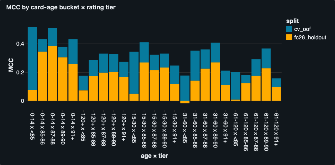
The skill is not evenly distributed. It concentrates on cards in the middle of their lifecycle, at higher rating tiers, and on evergreen cards whose value derives from card quality rather than a one-off event. The model is close to blind on event and promotion spikes: when a card jumps because a new promotion has launched, there is no signal for it, because the data contains no calendar of upcoming events. It is also weak on the low-priced segment that lies outside the training universe.
Two further limits. The edge holds at listed prices but becomes negative once about 2% friction per side is assumed, so it is an edge in the liquid part of the market rather than across all of it. And because only daily price history is available, the simulated trades are valued at known prices rather than verified fills; the simulation is strong evidence of the effect, not a brokerage record.
Conclusion
The system takes raw market data from several public sources, lands and cleans it in a reproducible Databricks lakehouse, and produces a price-direction model that clears its baselines, carries to a season excluded from training, and returns a positive result in a simulated portfolio after fees, with that result surviving a test against random selection. Trading the calls by hand for three weeks confirmed they can be filled at real prices, though that run is far too small to carry weight of its own. The main gaps are the absence of an event calendar, which would address the promotion spikes the model cannot currently see, and intra-trade pricing, which would tighten the portfolio simulation. The most promising follow-up is the exit rule: the live trades suggest the day-14 mark understates the signal, and re-running the backtest against exits inside the window would establish whether that holds.
Continuing into FC27. The model is now being tested on the live FC27 season: each week's calls are fingerprinted publicly before their outcomes are known, then revealed and scored as the weeks resolve, at vinaysankar2004.github.io/futvault-report/fc27.
Tools
Built on Databricks (Delta Lake, Unity Catalog, MLflow, and AI/BI dashboards) with Python for data collection and modeling, using scikit-learn and LightGBM for the models.